Code
librarian::shelf(readxl, data.table, DT, gt)

presets <- readxl::read_excel("R/pulse_presets.xlsx") |> as.data.table()
DT::datatable(presets, options = list(pageLength = 10, scrollX = TRUE))This document provides an overview of our current efforts in fitting “waveRAPID” data using the direct estimation method described in a 2020 patent (Fievet and Cottier 2020), and used in the publication by Kartal and colleagues (Kartal et al. 2021). The workflow includes the generation of fake experimental data, where necessary, smoothing, derivation, initial parameter estimation, nonlinear optimization, and bootstrapping for confidence interval determination.
The goal is to estimate kinetic parameters (\(k_a\), \(k_d\), \(R_{\text{max}}\)) from potentially noisy sensorgram data with a non-commercial approach, while assessing its robustness and reproducibility.
To generate fake, but realistic, experimental data, we first created an Excel file gathering the pulse presets available on the commercial system. The presets are defined for weak, intermediate and strong binders, and include the duration of each pulse, inter-dissociation time, last dissociation time, total time of the analysis, and acquisition frequency. To avoid typing mistakes, the total time of the analysis is actually re-calculated from the pulse durations and dissociation times prior to generating the fake data. A custom preset column was also included to allow for testing of custom pulse profiles.
librarian::shelf(readxl, data.table, DT, gt)
presets <- readxl::read_excel("R/pulse_presets.xlsx") |> as.data.table()
DT::datatable(presets, options = list(pageLength = 10, scrollX = TRUE))# Function to determine the current pulse
source("R/sim_waveRAPID.R")
# True parameters used for data simulation 1
ka <- 2710 # Association rate constant (M^-1 s^-1)
kd <- 0.278 # Dissociation rate constant (s^-1)
Rmax <- 14.77 # Maximum response (RU)
conc <- 100E-6 # Analyte concentration (M)
noise_sd <- 0.01 # Standard deviation of noise
cutoff_time <- 50 # Time cutoff for simulation (s)
# Simulate waveRAPID data using the defined parameters and the intermediate pulse preset,
# with a time cutoff of 50 seconds to focus on the most informative part of the response,
# and a random seed for reproducibility.
# The noise standard deviation is set to mimic realistic experimental conditions while allowing for parameter estimation.
sim <- simulate_waveRAPID(
true_ka = ka,
true_kd = kd,
true_Rmax = Rmax,
pulse_hgt = conc,
preset = "intermediate",
time_cutoff = cutoff_time,
seed = 42,
noise_sd = noise_sd,
file = "R/pulse_presets.xlsx"
)Fake experimental data was generated by simulating the response of a Langmuir binding model to a waveRAPID concentration profile. As a reminder, the concentration profile consists of multiple pulses of same concentration of analyte but increasing durations. The response is generated by solving the corresponding ordinary differential equation (ODE) with added noise to mimic experimental conditions.
Here, we developed an R function coined sim_waveRAPID, which i/ builds the pulse profile and concentration function \(c(t)\), then ii/ models the binding kinetics using the Langmuir model (Equation 1):
\[\frac{dR}{dt} = k_a \cdot c(t) \cdot (R_{\text{max}} - R) - k_d \cdot R \tag{1}\]
In this example, the parameters were set to \(c(t)=\) \(10^{-4}\), \(k_a =\) 2710, \(k_d =\) 0.278, and \(R_{\text{max}} =\) 14.77. The pulse starts and ends are those from the intermediate preset (Table 1). The signal was “collected” every 10 seconds over a total duration of 50 seconds (shorter than in the preset to focus on the most informative part of the response).
The ODE was solved using the ode function from the deSolve package, which provides a numerical solution for the response \(R(t)\) over time. The resulting response was then stored in a data table, and random noise was added with a normal distribution of standard deviation 0.01 to create a more realistic dataset for parameter estimation. The resulting kinetic data, presented in Figure 1, replicate faithfully the first example of Figure 4 from (Kartal et al. 2021).
sim_plot(sim) #plot simulated data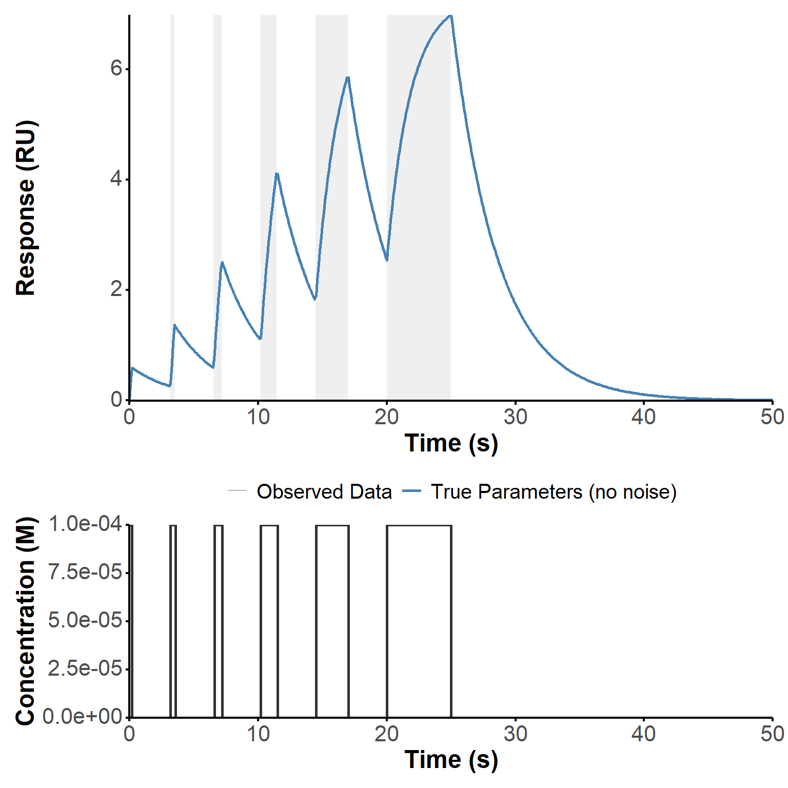
The following calculation and plotting were performed using the fit_waveRAPID function, which implements the smoothing and derivative estimation of data (Section 2.2.1), direct estimation method for waveRAPID data (Section 2.2.2), as well as nonlinear optimization for parameter refinement (Section 2.3). The function takes the simulated data as input, along with options for smoothing and regularization, and returns a fitted model object containing the estimated parameters and various diagnostic plots. The function is structured to allow for flexibility in the fitting process, including the choice of optimization method (OLS vs WLS) and the ability to perform bootstrapping for confidence interval estimation, using boot_waveRAPID (Section 2.3.2.2).
source("R/fit_waveRAPID.R") #function to fit

# Setup
smooth_value <- 0.01 # Smoothing parameter for the smoothing spline, set to a small value to allow for a close fit to the data while reducing noise-induced artifacts in the derivative estimation.
lbd <- 0   # Regularization parameter for the direct estimation method, set to 0 for no regularization in this initial fitting step. This can be tuned based on the level of noise and the desired balance between bias and variance in the parameter estimates.

fit <- fit_waveRAPID(
  sim_data = sim,
  do_optimization = FALSE,
  smooth_param = smooth_value,
  lbd = lbd
)
To estimate the kinetic parameters from the noisy response data, we first need to smooth the observed response and compute its derivative. The derivative will be used in the direct estimation method to construct the observation matrix and vector for parameter estimation. Noisy data can lead to artifacts in this derivative, so smoothing is essential to obtain reliable estimates. The influence of the smoothing parameter on the fit quality is further explored in Section 2.5.1, where we evaluate different values of the smoothing parameter in the context of increased noise in the data.
Here, we use a smoothing spline to fit the observed response_data and then compute the derivative of the smoothed response dR_dt (Figure 2).
fit_plot(fit, "deriv")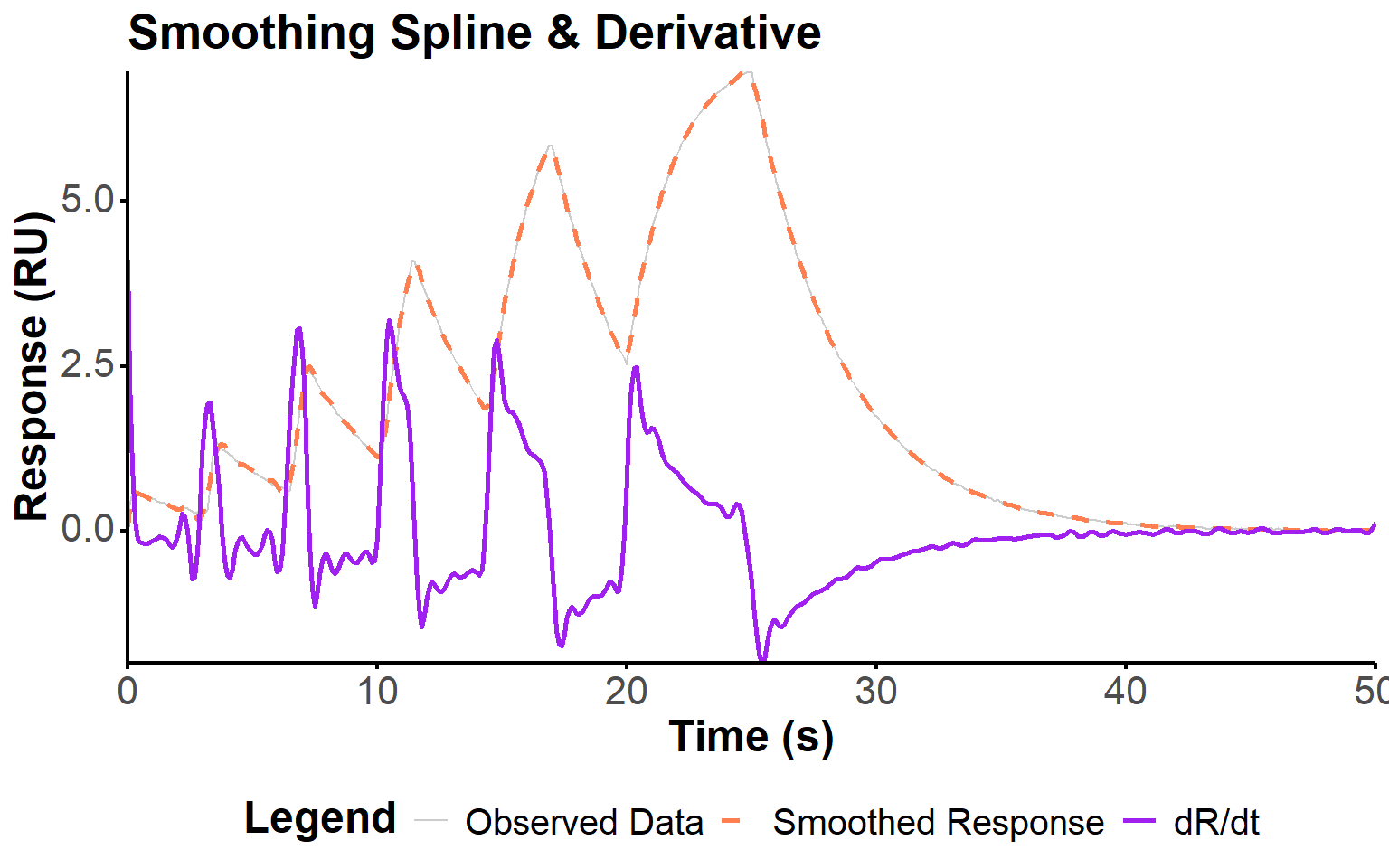
The direct estimation method for waveRAPID data involves constructing an observation matrix \(X\) and vector \(b\) from the smoothed response and its derivative. This approach is derived from the linearization of the Langmuir binding model, as described in the patent (Fievet and Cottier 2020). The observation matrix \(X\) is constructed as:
\[ X = \begin{bmatrix} -c(t) & c(t) \cdot \hat{R}(t) & \hat{R}(t) \end{bmatrix} \tag{2}\]
or more explicitely:
\[ X = \begin{bmatrix} -c_1 & c_1 \cdot \hat{R}_1 & \hat{R}_1 \\ \vdots & \vdots & \vdots \\ -c_n & c_n \cdot \hat{R}_n & \hat{R}_n \end{bmatrix} \tag{3}\]
where:
The observation vector \(b\) is simply the derivative of the smoothed response \(\frac{d\hat{R}}{dt}\): \[ b = \begin{bmatrix} (\frac{d\hat{R}}{dt})_1 \\ \vdots \\ (\frac{d\hat{R}}{dt})_n \end{bmatrix} \tag{4}\]
The intermediate parameters \(\theta = [\theta_1, \theta_2, \theta_3]^T\) are estimated by solving the regularized linear system:
\[ \hat{\theta} = -(X^T X + \Lambda I)^{-1} X^T b \tag{5}\]
where \(\Lambda\) is a regularization parameter to stabilize the solution. This follows the principle of Tikhonov regularization (also called Ridge regression), which is commonly used to estimate coefficients in multiple-regression problems, especially when the variables are highly correlated.
Here \(\Lambda\) is a diagonal matrix with \(\lambda\) on the diagonal. This regularization term may help to prevent overfitting and ensure that the parameter estimates are stable, especially when the observation matrix \(X\) is ill-conditioned or when there is significant noise in the data. \(\lambda\) (and therefore \(\Lambda\)) can be tuned based on the level of noise and the desired balance between bias and variance in the parameter estimates. It was here kept at 0, but its influence is studied in Section 2.5.2.
The kinetic parameters are then recovered as:
\[ k_a = \theta_2, \quad k_d = \theta_3, \quad R_{\text{max}} = \frac{\theta_1}{\theta_2} \tag{6}\]
Here, we found the following values for the kinetic parameters:
\(k_a =\) 1498, \(k_d =\) 0.2583, and \(R_{\text{max}} =\) 17.02.
Note that R was artifically decreased to 80% of its estimated value, as more accurate estimations produced issues with the optimization step, below. Hence, the corresponding simulation of the response using the ODE model does not match the experimental response intensity (Figure 3). However, the kinetic parameters are close to the true parameters, and the shape of the response is reasonably well captured, which is sufficient for the optimization step.
fit_plot(fit, "init_estim")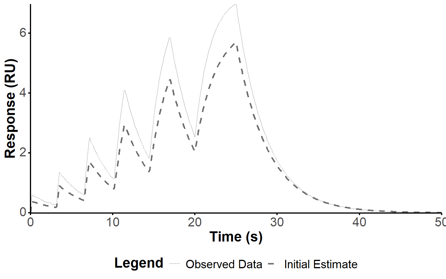
fit <- fit_waveRAPID(
  sim_data = sim,
  do_optimization = TRUE,
  smooth_param = smooth_value,
  lbd = lbd
)
To further refine the parameter estimates obtained from the direct estimation method, we can perform nonlinear optimization using ordinary least squares (OLS) or weighted least squares (WLS) fitting. The objective function is defined as the sum of squared residuals (SSR) between the observed response and the predicted response from the ODE simulation.
\[ SSR_{\text{OLS}} = \sum_{i=1}^{n} (R_{\text{obs}, i} - R_{\text{pred}, i})^2 \tag{7}\]
Here, we chose to optimize the parameters in log-space to ensure positivity and to handle the wide range of parameter values effectively during optimization. Hence, the log_objective_function takes the log-transformed parameters, simulates the response using the ODE model, and computes the SSR. The ODE is solved with the lsoda method, which automatically handles stiff and non-stiff problems, and we set tolerances and maximum steps to ensure a balance between accuracy and computational efficiency. We leveraged the R implementation included in the deSolve package (Soetaert, Petzoldt, and Setzer 2010), which interfaces with the underlying Fortran code (Petzold 1983).
If the dissoc_only flag is set to TRUE, the optimization switches to WLS by by assigning zero weights to the association phases in the SSR calculation, and therefore focuses on dissociation data only. This is suggested in the original publication to avoid RI disturbance (Kartal et al. 2021), so that misfits in the association parts of the pulses do not impact the parameter estimation. Concretely, we defined association and dissociation phases based on the concentration profile, where association phases correspond to times when \(c(t)\) is greater than zero and dissociation phases correspond to times when \(c(t)\) is nil. Equation Equation 7 is therefore modified to include weights as follows:
\[ SSR_{\text{WLS}} = \sum_{i=1}^{n} w_i (R_{\text{obs}, i} - R_{\text{pred}, i})^2 \tag{8}\]
where \(w_i\) is the weight for each time point, defined as: \[w_i = \begin{cases}0 & \text{if } c(t_i) > 0 \quad (\text{association phase}) \\1 & \text{if } c(t_i) = 0 \quad (\text{dissociation phase})\end{cases} \tag{9}\]
The optimization is performed using the COBYLA algorithm (Constrained Optimization BY Linear Approximations) for derivative-free optimization with nonlinear inequality and equality constraints. We used the R implementation of COBYLA available in the nloptr package (Ypma and Johnson 2011) (an R interface to the NLOPT library (Johnson 2026)), adapted from Jean-Sébastien Roy’s C implementation of the original Fortran code by M. J. D. Powell (Powell 1994). Other algorithm are tested, on real data, further down this document (Section 3.4).
The optimization is bounded around the initial estimates to ensure that the parameter search is focused and to prevent divergence. Below is shown the default output of the fit function, including the number of iterations, the final parameter estimates, and the value of the objective function at the optimum.
fit── waveRAPID_fit ──────────────────────────────────────────
Stages run : 1, 2, 3
True params : ka = 2710 | kd = 0.278 | Rmax = 14.77
Initial estim : ka = 1497.54 | kd = 0.258332 | Rmax = 17.0173
OLS : ka = 2269.83 | kd = 0.280808 | Rmax = 16.7971
Convergence : status = 4 | iter = 99 | obj = 0.967274
Message : NLOPT_XTOL_REACHED: Optimization stopped because xtol_rel or xtol_abs (above) was reached.
WLS : ka = 2487.79 | kd = 0.281455 | Rmax = 15.8079
Convergence : status = 4 | iter = 169 | obj = 0.175332
Message : NLOPT_XTOL_REACHED: Optimization stopped because xtol_rel or xtol_abs (above) was reached.
Residual summary (sd):
OLS sd = 0.0389
WLS sd = 0.0290
Available plots: obs, deriv, init_estim, fit, comparison, residuals
───────────────────────────────────────────────────────────Table 2 presents the kinetic parameters obtained from the initial estimation, OLS optimization, and WLS optimization, along with their comparison to the true parameters used for data simulation. The table also includes the percentage of the true parameters represented by the initial estimates and the optimized estimates for both approaches. WLS allows the closest estimation of the true values; in particular the improvement of the association constant is significant. The \(R_{\text{max}}\) value is also closer to reality.
These refined estimates of the kinetic parameters were used to simulate the response, and compare it to the observed data for visual validation (Figure 4). The slight overestimation of \(R_{\text{max}}\) by OLS is visible but modest, and the fits are generally visually excellent.
get_param_table(fit)fit_plot(fit, "fit")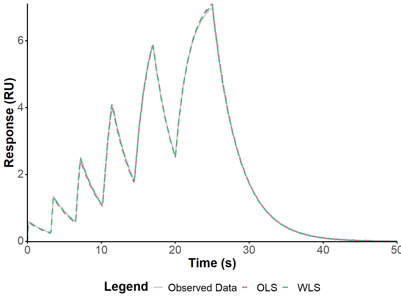
Residuals are a key diagnostic tool for assessing the quality of the fit and identifying any systematic deviations between the observed data and the model predictions. They were calculated as the difference between the observed response and the predicted response from the ODE simulation using the estimated parameters. The residuals were then plotted over time to visually inspect for patterns, trends, or heteroscedasticity, which may indicate model misspecification or areas where the fit could be improved. Figure 5 shows an improvement in the residuals using WLS, as expected from the observations above. However, these residuals do not seem to be normally distributed.
Q-Q plots can help to identify any deviations from normality, such as skewness or heavy tails, which could impact the validity of the parameter estimates and the confidence intervals derived from them. In particular, OLS optimizations assumes that the residuals are normally distributed. Here, the points in the OLS Q-Q plot deviate substantially from the dashed reference line, especially at both tails (lower and upper quantiles), suggesting that the residuals are not normally distributed. This may be due to the influence of RI during association phases. In contrast, the WLS Q-Q plot shows points that are much closer to the reference line, indicating that the residuals from the WLS fit are more normally distributed. There is still some deviation, particularly in the lower quantiles. Other approaches to opmitization could be explored to further improve the fit and the normality of the residuals, such as using more robust regression methods (e.g., Huber regression, Tukey’s bisquare). Generalized least squares (GLS) could also be considered to account for any heteroscedasticity in the residuals, by explicitely modeling their covariance structure.
fit_plot(fit, "residuals")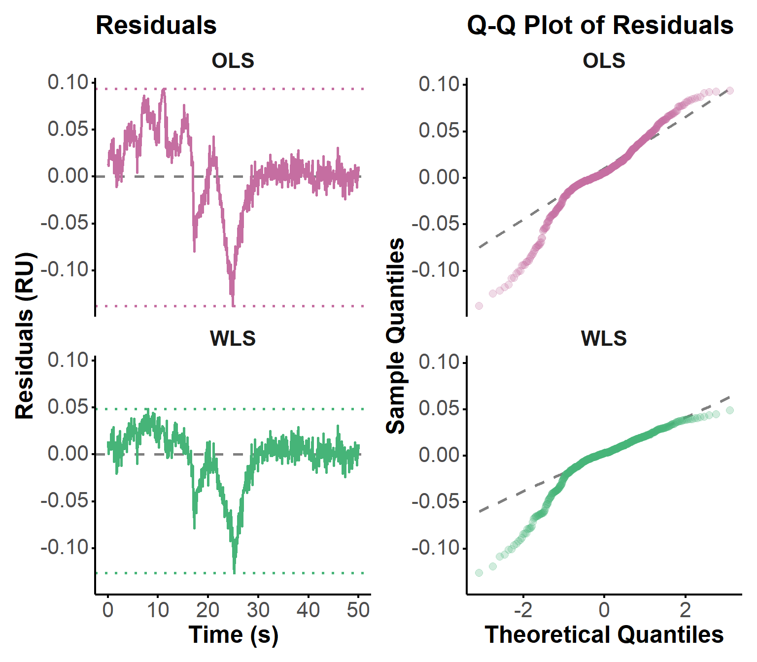
Finally, we performed non-parametric bootstrapping analysis to provide a robust estimate of the uncertainty in the kinetic parameters. The principle of bootstrapping is to assess the variability of parameter estimates by resampling the observed data with replacement and re-estimating the parameters for each bootstrap sample. This approach allows us to derive confidence intervals for the parameters without relying on strict parametric assumptions, which is particularly useful in complex models like ours where the distribution of parameter estimates may not be normal.
Practically, we generated bootstrap samples by resampling the residuals from the best-fitting model (using WLS) and adding them back to the smoothed response. For each bootstrap sample, we re-estimated the parameters using the same RAPID linear approach followed by nonlinear refinement with COBYLA. We carried out 100 iterations to balance accuracy and computational time. To significantly decrease the latter, we implemented the bootstrap procedure in parallel on multiple CPU cores using the parallel package.
The resulting distributions of parameter estimates across all bootstrap iterations were then summarized to obtain median values and 95% confidence intervals for each parameter (Table 3).
param_table(boot) The bootstrap distributions are also shown as density plots, showing the true parameter values (dashed blue lines), the median of the bootstrap estimates (dashed pink), and the 95% confidence intervals (dotted pink; Figure 6).
plot(boot, "density")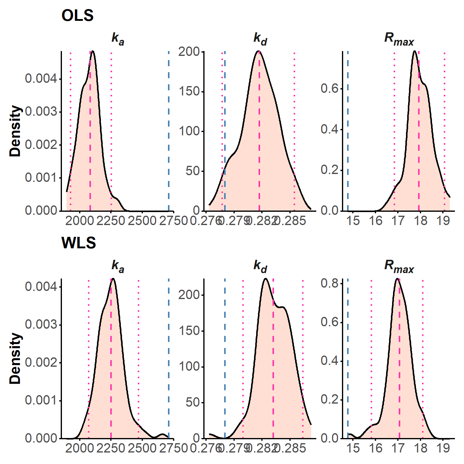
Additionally, we plotted the correlation between the bootstrap estimates of \(k_a\) and \(k_d\), colored by \(R_{\text{max}}\), to explore any potential relationships between the parameters across the bootstrap iterations (Figure 7). The somewhat linear relationship that is observed between \(k_a\), \(k_d\) and \(R_{\text{max}}\) across the OLS bootstrap iterations is indicative of a potential trade-off between these parameters, which is not surprising given that they are linked by the \(K_d\).
plot(boot, "scatter")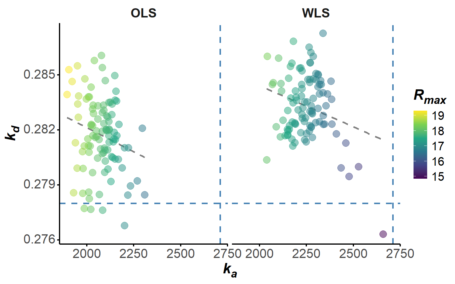
Below, we apply the same approach to the two other experiments shown in Figure 4 from the original publication (Kartal et al. 2021). Relatively good fits are obtained, with a significant improvement when using WLS.
ka_2 <- 1.16E4
kd_2 <- 4.60E-2
Rmax_2 <- 26.30
conc_2 <- 10E-6
noise_sd_2 <- 0.01
cutoff_time_2 <- 50

ka_3 <- 8.40E3
kd_3 <- 5.50E-3
Rmax_3 <- 25.80
conc_3 <- 10E-6
noise_sd_3 <- 0.01
cutoff_time_3 <- 50 fit_2 <- fit_waveRAPID(
sim_data = simulate_waveRAPID(
true_ka = ka_2,
true_kd = kd_2,
true_Rmax = Rmax_2,
pulse_hgt = conc_2,
preset = "intermediate",
time_cutoff = cutoff_time_2,
seed = 42,
noise_sd = noise_sd_2,
file = "R/pulse_presets.xlsx"
),
do_optimization = TRUE,
smooth_param = smooth_value,
lbd = lbd
)
fit_3 <- fit_waveRAPID(
sim_data = simulate_waveRAPID(
true_ka = ka_3,
true_kd = kd_3,
true_Rmax = Rmax_3,
pulse_hgt = conc_3,
preset = "intermediate",
time_cutoff = cutoff_time_3,
seed = 42,
noise_sd = noise_sd_3,
file = "R/pulse_presets.xlsx"
),
do_optimization = TRUE,
smooth_param = smooth_value,
lbd = lbd
)fit_plot(fit_2, "fit")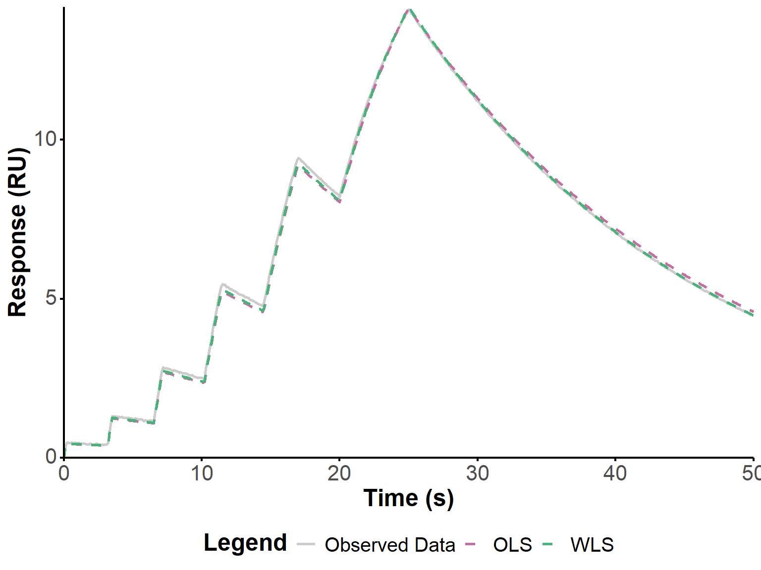
get_param_table(fit_2)fit_plot(fit_3, "fit")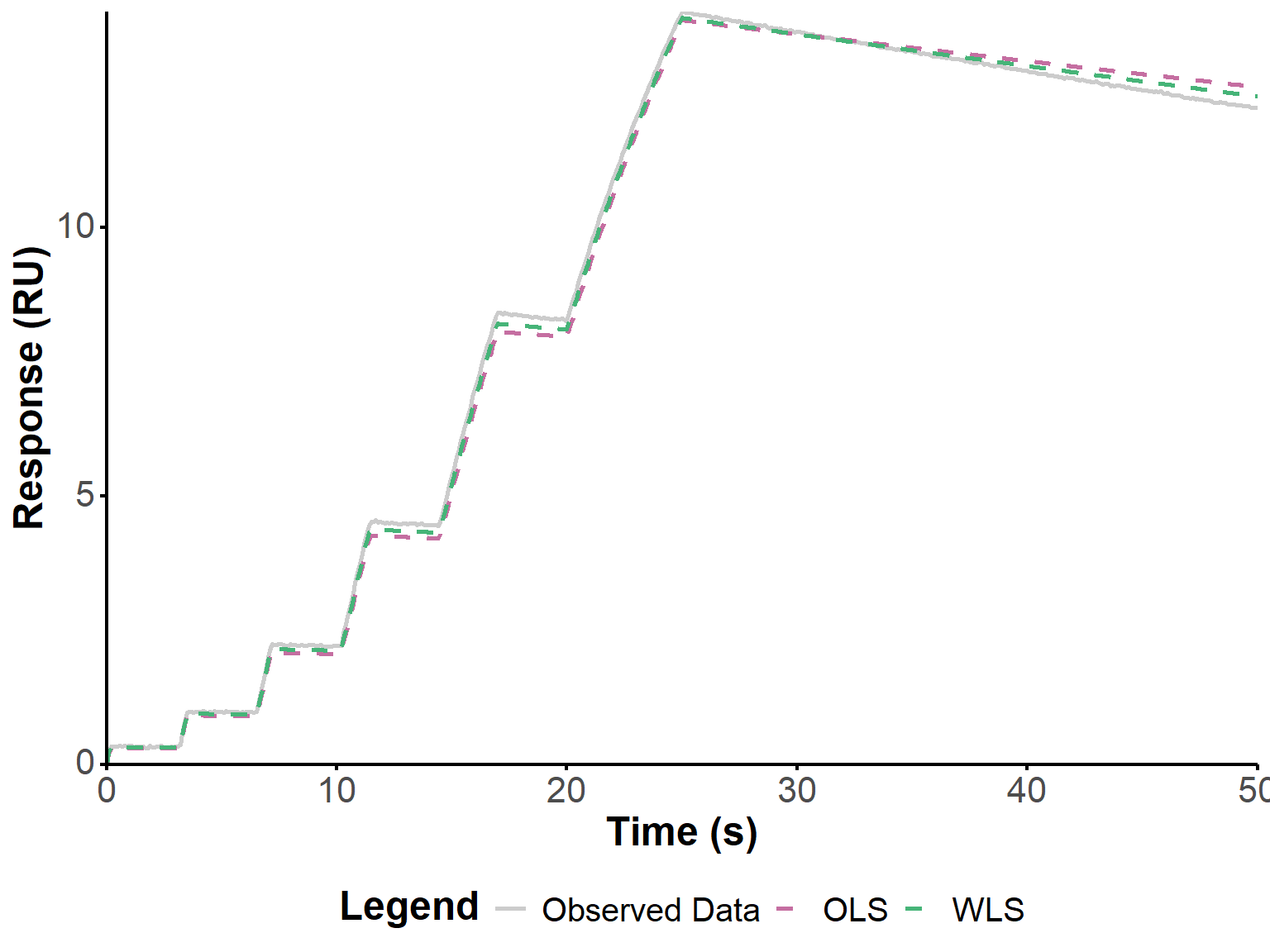
get_param_table(fit_3)boot_2 <- boot_waveRAPID(fit_2, n_boot = n_boot)boot_3 <- boot_waveRAPID(fit_3, n_boot = n_boot)In this last example, we reproduce the data from the first example but with 10 times more noise (Figure 10), to better evaluate the robustness of the approach to noise, and the potential improvement brought by WLS.
# True parameters used for data simulation 1
ka <- 2710          # Association rate constant (M^-1 s^-1)
kd <- 0.278         # Dissociation rate constant (s^-1)
Rmax <- 14.77       # Maximum response (RU)
conc <- 100E-6      # Analyte concentration (M)
noise_sd <- 0.1     # Standard deviation of noise (10 times higher)
cutoff_time <- 50   # Time cutoff for simulation (s)

# Simulate waveRAPID data using the defined parameters and the intermediate pulse preset,
# with a time cutoff of 50 seconds to focus on the most informative part of the response,
# and a random seed for reproducibility.
# The noise standard deviation is set to mimic realistic experimental conditions while allowing for parameter estimation.
sim_noise <- simulate_waveRAPID(
  true_ka = ka,
  true_kd = kd,
  true_Rmax = Rmax,
  pulse_hgt = conc,
  preset    = "intermediate",
  time_cutoff = cutoff_time,
  seed      = 42,
  noise_sd  = noise_sd,
  file = "R/pulse_presets.xlsx"
)#+ label: fig-noise
#| fig-cap: "Simulated waveRAPID data with increased noise, showing the observed response (with higher noise) and the concentration profile over time. Blue ribbons indicate the association phases (when the analyte is present), while white areas indicate the dissociation phases (when the analyte is absent).
#| fig-height: 8
sim_plot(sim_noise)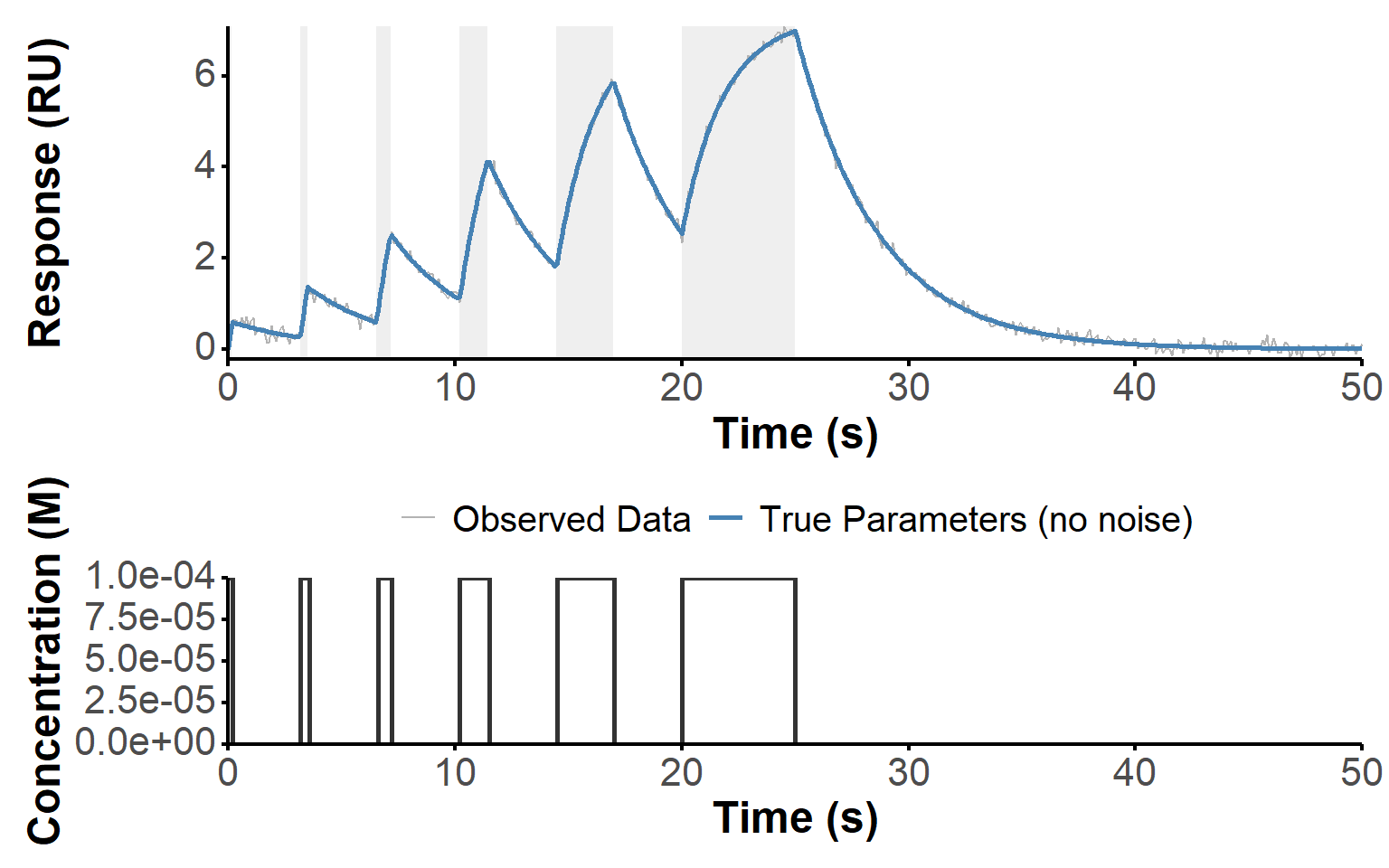
We use below three smoothing parameters values, spanning three orders of magnitudes, to evaluate the influence of this parameter on the fit quality in the context of increased noise in the data. The regularization parameter is kept at 0 to focus on the impact of smoothing only.
The fit quality is visually similar (Figure 11) for the different smoothing parameters, and the estimated values are generally very close. The largest smoothing value (0.1) seems to produce a slightly worse fit, and a slightly worse estimation of the kinetic parameters, but the differences are not very significant. The WLS approach seems to be more robust to estimate the association constant, which in any case remains relatively far from the true value.
smooth_values <- c(0, 0.001, 0.01, 0.1)
captions <- paste("Smoothing parameter:", smooth_values)
lbd <- 0

fit_noises <- lapply(smooth_values, function(x) {
  fit_waveRAPID(
    sim_data = sim_noise,
    do_optimization = TRUE,
    smooth_param = x,
    lbd = 0
  )
})

p_noise_1 <- (fit_plot(fit_noises[[1]], "deriv") + ggtitle(captions[1])) /
  (fit_plot(fit_noises[[2]], "deriv") + ggtitle(captions[2])) /
  (fit_plot(fit_noises[[3]], "deriv") + ggtitle(captions[3])) /
(fit_plot(fit_noises[[4]], "deriv") + ggtitle(captions[4]))p_noise_2 <- (fit_plot(fit_noises[[1]], "fit") + ggtitle(captions[1])) /
(fit_plot(fit_noises[[2]], "fit") + ggtitle(captions[2])) /
(fit_plot(fit_noises[[3]], "fit") + ggtitle(captions[3])) /
(fit_plot(fit_noises[[4]], "fit") + ggtitle(captions[4]))p_noise_1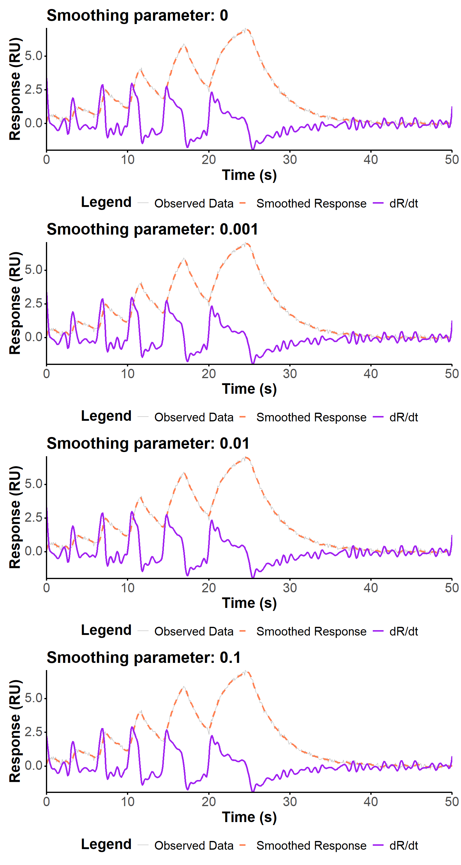
p_noise_2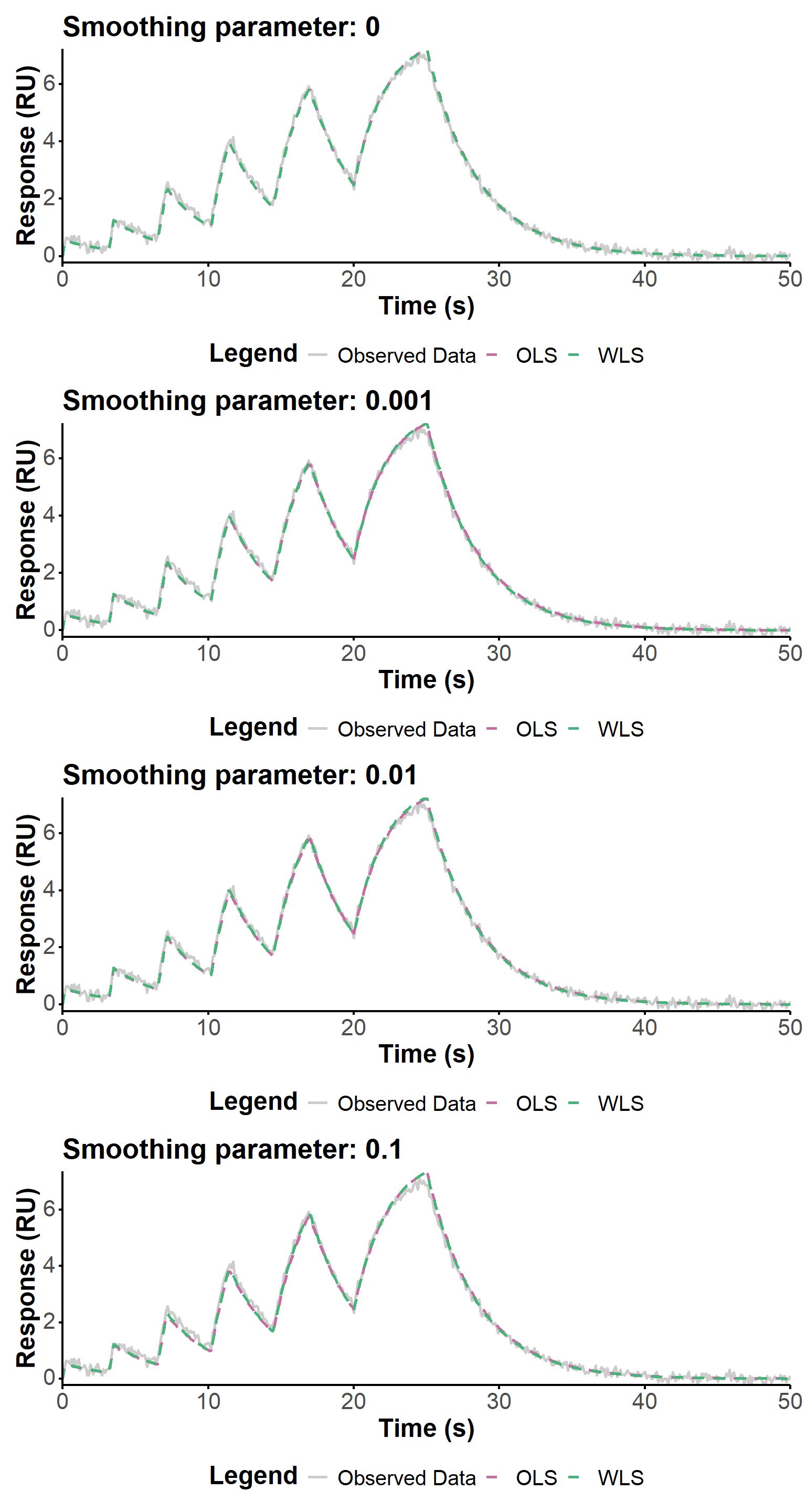
tbl_noises <- lapply(fit_noises, function(fitty) {
  get_param_table(fitty)
})

tbl_noises[[1]]
tbl_noises[[2]]
tbl_noises[[3]]
tbl_noises[[4]]Here, we use four values of the regularization parameter, spanning several orders of magnitude, to evaluate the influence of this parameter on the fit quality in the context of increased noise in the data. The smoothing parameter is kept at 0.01 to focus on the impact of regularization only. The fit quality is visually similar (Figure 12) for \(\lambda \ll 10^{-6}\), and the estimated values are generally very close. The largest regularization value (\(\lambda = 10^{-6}\)) fails to fit correctly the data.
smooth_value <- 0.01
lbds <- c(0, 1E-12, 1E-9, 1E-6)
captions <- paste("Λ =", lbds)
fit_lbds <- lapply(lbds, function(x) {
fit_waveRAPID(
sim_data = sim_noise,
do_optimization = TRUE,
smooth_param = smooth_value,
lbd = x
)
})
p_lambda_2 <- (fit_plot(fit_lbds[[1]], "fit") + ggtitle(captions[1])) /
(fit_plot(fit_lbds[[2]], "fit") + ggtitle(captions[2])) /
(fit_plot(fit_lbds[[3]], "fit") + ggtitle(captions[3])) /
(fit_plot(fit_lbds[[4]], "fit") + ggtitle(captions[4]))p_lambda_2 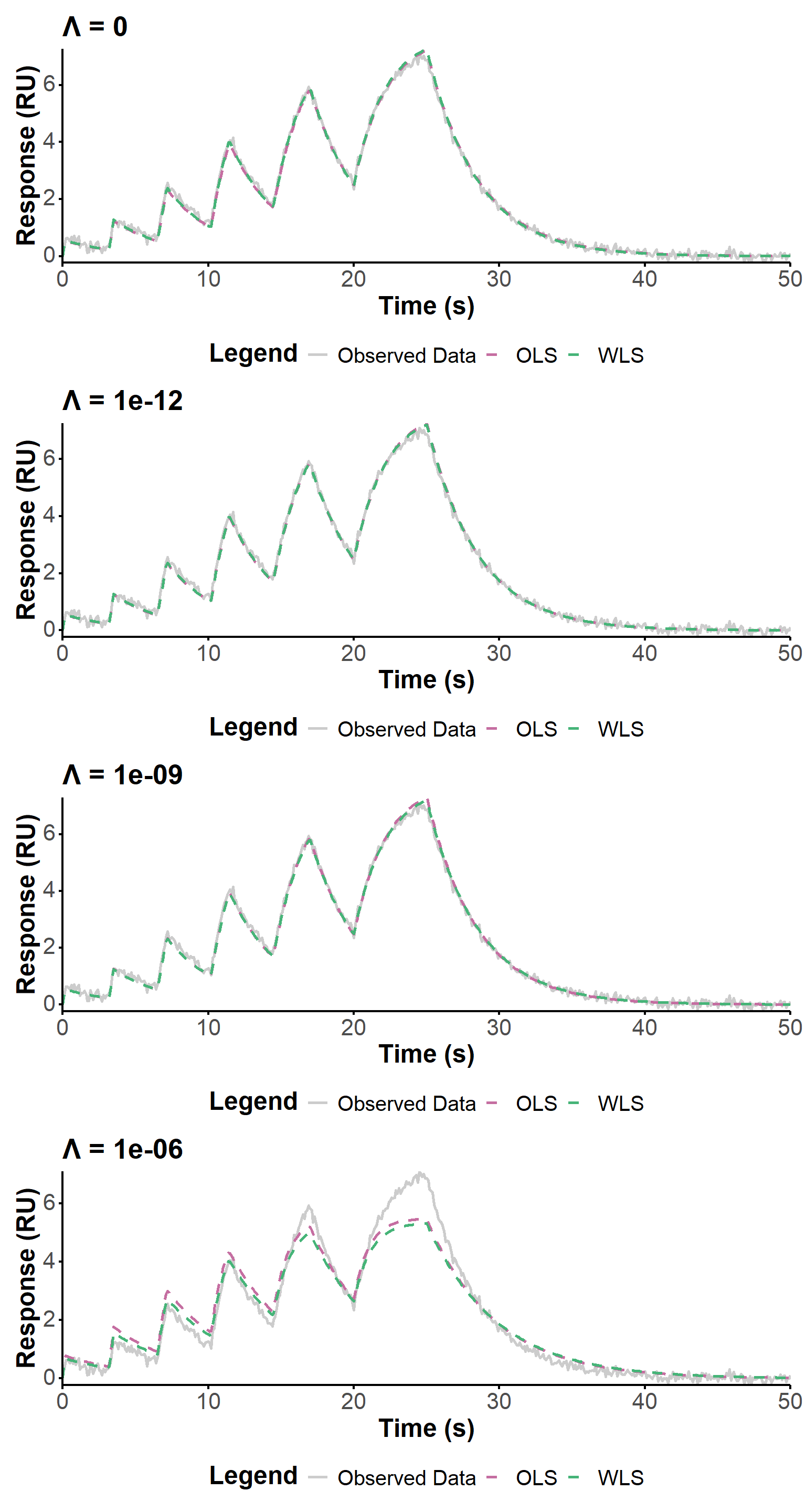
tbl_lbds <- lapply(fit_lbds, function(fitty) {
  get_param_table(fitty)
})

tbl_lbds[[1]]
tbl_lbds[[2]]
tbl_lbds[[3]]
tbl_lbds[[4]]Overall, we have successfully implemented the direct estimation method for fitting waveRAPID data, as described in the original patent and publication. The approach allows for the estimation of kinetic parameters from noisy sensorgram data, with the option to focus on dissociation phases to mitigate RI effects. The use of bootstrapping provides a robust way to assess the uncertainty in the parameter estimates. Future work could explore alternative optimization methods to further improve the fit quality and parameter estimation, especially in the context of high noise levels.
We look here at data acquired with biolayer interferometry (BLI), using only 4 pulses (coined hereafter as RAPID4). Three different analyte concentrations were tested (500 nM, 1 µM, 2 µM). The fitting script was modified to allow for i/ handling experimental data, ii/ accepting custom pulse profiles with fewer than 6 pulses, iii/ optionally optimizing on the smoothed data rather than the raw data to increase the accuracy and speed of processing, and iv/ choosing the optimization algorithm, in addition to the default COBYLA.
First, we simulated the response of the system to the custom pulse profiles used in the experiments, using the simulate_waveRAPID function with the corresponding parameters for each experiment, and the optimized parameters obtained on the Biacore instrument (Figure 13). This allows us to have a theoretical reference for the expected response based on the known kinetic parameters and pulse profiles, which can be useful for validating the fitting procedure and interpreting the results from the experimental data.
# Simulation of theoretical data====
sim_param <- data.table(
  exp = c("2 µM", "1 µM", "500 nM"),
  conc = c(2e-6, 1e-6, 0.5e-6),
  kon = c(9.8e4, 1.15e5, 1.3e5),
  koff = c(0.0125, 0.0133, 0.0126),
  R_max = c(0.106, 0.0948, 0.085),
  time_cutoff = c(350, 350, 350)
)

preset <- "custom"

sim_mck <- lapply(
  unique(sim_param$exp),
  function(experiment) {
    params <- sim_param[exp == experiment]
    simulate_waveRAPID(
      true_ka = params$kon,
      true_kd = params$koff,
      true_Rmax = params$R_max,
      pulse_hgt = params$conc,
      preset = preset,
      time_cutoff = params$time_cutoff,
      seed = 42,
      noise_sd = 0,
      file = "R/pulse_presets_2.xlsx"
    )
  }
)

# name the list elements according to the experiment
names(sim_mck) <- unique(sim_param$exp)

patchwork::wrap_plots(
  sim_plot(sim_mck[["2 µM"]]),
  sim_plot(sim_mck[["1 µM"]]),
  sim_plot(sim_mck[["500 nM"]])
) +
  plot_layout(guides = "collect", ncol = 1) &
theme(legend.position = "bottom") 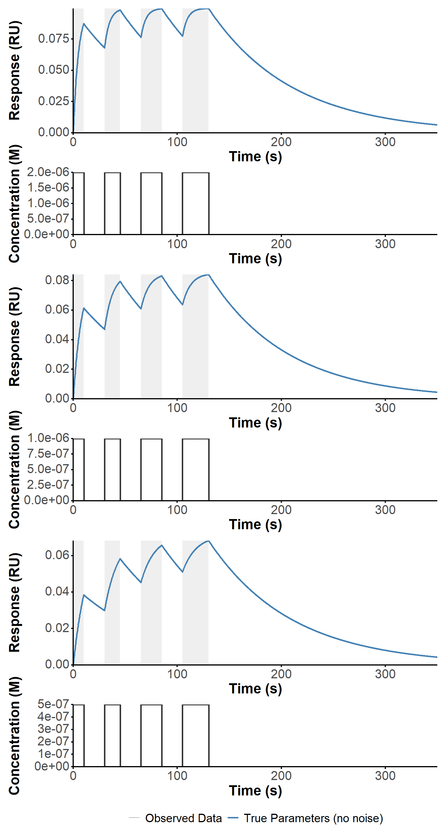
An offset of 60 seconds was applied to the time axis to account for the delay between the start of the acquisition and that of the first pulse (Figure 14). The raw data files were imported and pre-processed to extract the relevant columns (time and signal), filter out any rows with missing values, and create a long-format data table that combines all experiments for subsequent analysis and plotting.
## Parameters====

custom_theme <- theme_minimal() +
  theme(
    axis.line = element_line(size = 0.75, color = "black"),
    axis.ticks = element_line(size = 0.75, color = "black"),
    axis.title = element_markdown(size = 18, face = "bold"),
    axis.text = element_markdown(size = 16),
    legend.text = element_text(size = 15),
    legend.title = element_markdown(size = 18, face = "bold"),
    legend.position = "right",
    strip.text.x = element_markdown(size = 16, face = "bold"),
    strip.text.y = element_markdown(size = 16, face = "bold"),
    panel.grid = element_blank(),
    plot.title = element_markdown(size = 20, face = "bold"),
    plot.subtitle = element_markdown(size = 16)
  )

time_offset <- 60 # s

## Data import and pre-processing====

file_list <- list.files("BLI/raw_data", pattern = "RAPID4", full.names = TRUE)

long_dt <- lapply(
  file_list,
  function(file) {
    dt <- fread(
      file,
      col.names = c(
        "time_1",
        "signal_1",
        "fit_time_2",
        "fit_signal_2"
      )
    ) |>
      _[, .SD, .SDcols = !patterns("fit")] |>
      _[!is.na(signal_1)] |>
      _[, exp := gsub(".*RAPID4 (.*)\\.txt", "\\1", file)] |>
      _[, .(time = time_1 - time_offset, R_t_obs = signal_1, exp)][
        time >= 0
      ]

    sim_mck_exp <- sim_mck[[unique(dt$exp)]]

    dt <- dt[1:(nrow(sim_mck_exp@response_data))]
  }
) |>
  rbindlist() |>
  _[,
    exp := fcase(
    exp == "2uM", "2 µM",
    exp == "1uM", "1 µM",
    exp == "500 nM", "500 nM"
  )
  ]


ggplot(long_dt,
aes(x = time, y = R_t_obs, color = factor(exp))) +
  geom_line(linewidth = 1) +
  labs(x = "Time (s)", y = "Observed response (RU)", color = "Experiment") +
  custom_theme +
  theme(legend.position = "bottom") +
scale_color_manual(values = c("#1b9e77", "#d95f02", "#7570b3")) 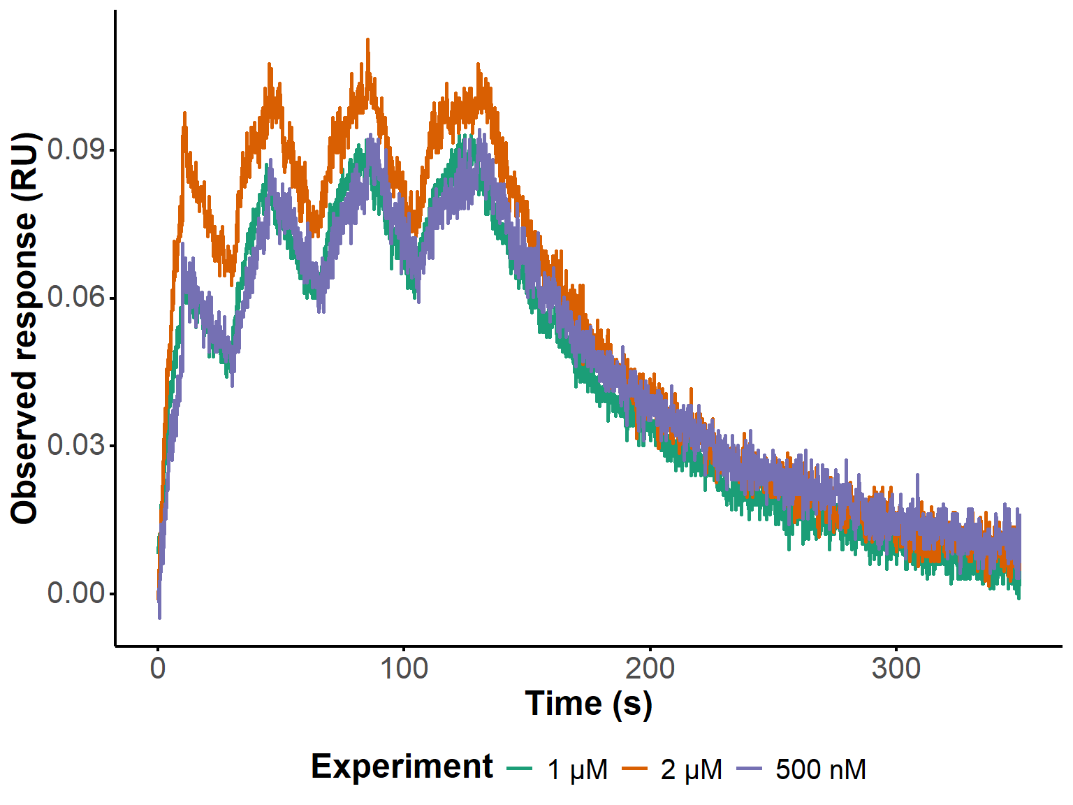
After successfully fitting all three experiments with default parameters (not shown, for brevity), we evaluated the influence of the smoothing parameter on the fit quality and parameter estimation. We tested 10 different values of the smoothing parameter, ranging from 0.1 to 1, and compared the percentage error of the estimated kinetic parameters for both OLS and WLS models (Figure 15).
For the experiments at 2 µM and 1 µM, little variations are observed below 0.6, with generally excellent agreement with the Biacore estimates.
At 500 nM however, for which much larger errors are observed, conflicting results are observed. The Rmax estimation improves with increasing smoothing, while the kd estimation worsens (similar to what is observed at 1 and 2 µM). Finally, the estimation of ka worsens with increasing smoothing for the OLS model, while it improves for the WLS model, for which the estimation at low smoothing is particularly bad.
In the case at hand, it seems that smoothing values around 0.5 should provide the best compromise for the estimation of all parameters. However, this is obsviously S/N dependent and for not too challenging datasets, the impact of the smoothing parameter on the estimation accuracy is rather modest. In other words, the optimization of kinetic parameters is generally robust, and the smoothing parameters may need to be carefully tuned for particularly noisy data only.
smooth_comp_param_store <- smooth_comp_param_store[,
param := fcase(
  param == "ka", "<i>k</i><sub>a</sub>",
  param == "kd", "<i>k</i><sub>d</sub>",
  param == "Rmax", "<i>R</i><sub>max</sub>"
)
]


ggplot(
  smooth_comp_param_store,
  aes(x = as.numeric(smooth_param), y = pct_error, color = model)
) +
  geom_line(linewidth = 1) +
  geom_point(size = 4) +
  geom_point(
    data = smooth_comp_param_store[,
      .SD[which.min(pct_error)],
      by = .(experiment, model, param)],
    aes(x = as.numeric(smooth_param), y = pct_error, color = model),
    size = 5,
    shape = 21,
    fill = "white",
    stroke = 1.5,
    show.legend = FALSE
  ) +
  facet_grid(param ~ experiment) +
  labs(x = "Smoothing Parameter", y = "% Error", color = "Model") +
  theme_minimal() +
  scale_color_manual(values = c("OLS" = "#c56ea1", "WLS" = "#46b478")) +
  scale_x_continuous(breaks = smooth_list[(smooth_list * 10) %% 2 == 0]) +
  custom_theme +
  theme(legend.position = "bottom")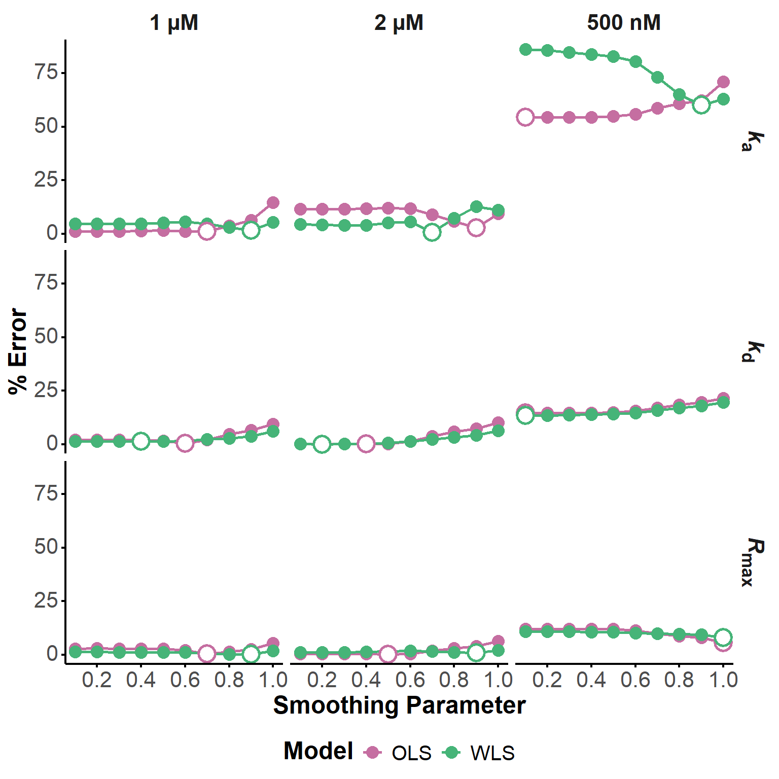
Here, we compared the optimized parameter estimates obtained with six different local derivative-free optimization algorithms from the NLOPT library (Johnson 2026), namely COBYLA (Powell 1994), BOBYQA (Powell 2009), NEWUOA (Powell 2004), PRAXIS (PRincipal AXIS) (Brent 1972), Nelder-Mead Simplex (Nelder and Mead 1965; Box 1965), and SBPLX (based on Subplex (Rowan)). In all cases, bound constraints were used; even if not originally included in some of these algorithms, they are always available in their NLOPT implementations.
The percentage error of the estimated kinetic parameters was calculated for each algorithm and model, and the results are grouped in Table 8. The differences are marginal, as can also be seen in Figure 16. As in the case of smoothing, the workflow is robust and does not depend significantly on the choice of the optimization algorithm, at least for this dataset.
#|
gt_algo_comp <- algo_comp_param_store[,
  algorithm := gsub("NLOPT_LN_", "", algorithm)
] |>
  _[order(param, experiment, model, algorithm)] |>
  _[, param_exp_grp := paste0(param, " | ", experiment, " | Reference value: ", true_value)] |>
  as.data.frame() |>
  gt(groupname_col = "param_exp_grp") |>
  cols_hide(c("param", "experiment", "true_value")) |>
  fmt_scientific(columns = "value", decimals = 3) |>
  fmt_scientific(columns = "true_value", decimals = 3) |>
  fmt_number(columns = "pct_error", decimals = 2) |>
  data_color(
    columns = "pct_error",
    colors = scales::col_numeric(
      palette = c("forestgreen", "white", "coral"),
      domain = c(0, 5),
      na.color = "coral",
      alpha = 0.8
    )
  ) |>
  cols_label(
    algorithm = html("<b>Algorithm</b>"),
    model = html("<b>Model</b>"),
    value = html("<b>Estimated Value</b>"),
    true_value = html("<b>True Value</b>"),
    pct_error = html("<b>% Error</b>")
  ) |>
  # tab_header(title = html("<b>Algorithm Comparison: Parameter Estimation</b>")) |>
  tab_style(
    style = cell_text(weight = "bold"),
    locations = cells_row_groups()
  ) |>
  opt_row_striping()

gt_algo_comp| Algorithm | Model | Estimated Value | % Error |
|---|---|---|---|
| Rmax | 1 µM | Reference value: 0.0948 | |||
| BOBYQA | OLS | 9.748 × 10⁻² | 2.82 |
| COBYLA | OLS | 9.750 × 10⁻² | 2.85 |
| NELDERMEAD | OLS | 9.748 × 10⁻² | 2.83 |
| NEWUOA_BOUND | OLS | 9.748 × 10⁻² | 2.82 |
| PRAXIS | OLS | 9.749 × 10⁻² | 2.83 |
| SBPLX | OLS | 9.749 × 10⁻² | 2.84 |
| BOBYQA | WLS | 9.367 × 10⁻² | 1.19 |
| COBYLA | WLS | 9.372 × 10⁻² | 1.14 |
| NELDERMEAD | WLS | 9.367 × 10⁻² | 1.19 |
| NEWUOA_BOUND | WLS | 9.368 × 10⁻² | 1.18 |
| PRAXIS | WLS | 9.368 × 10⁻² | 1.18 |
| SBPLX | WLS | 9.369 × 10⁻² | 1.18 |
| Rmax | 2 µM | Reference value: 0.106 | |||
| BOBYQA | OLS | 1.064 × 10⁻¹ | 0.33 |
| COBYLA | OLS | 1.064 × 10⁻¹ | 0.34 |
| NELDERMEAD | OLS | 1.064 × 10⁻¹ | 0.33 |
| NEWUOA_BOUND | OLS | 1.064 × 10⁻¹ | 0.33 |
| PRAXIS | OLS | 1.064 × 10⁻¹ | 0.33 |
| SBPLX | OLS | 1.064 × 10⁻¹ | 0.34 |
| BOBYQA | WLS | 1.046 × 10⁻¹ | 1.35 |
| COBYLA | WLS | 1.046 × 10⁻¹ | 1.33 |
| NELDERMEAD | WLS | 1.046 × 10⁻¹ | 1.35 |
| NEWUOA_BOUND | WLS | 1.046 × 10⁻¹ | 1.36 |
| PRAXIS | WLS | 1.046 × 10⁻¹ | 1.35 |
| SBPLX | WLS | 1.046 × 10⁻¹ | 1.35 |
| Rmax | 500 nM | Reference value: 0.085 | |||
| BOBYQA | OLS | 9.523 × 10⁻² | 12.00 |
| COBYLA | OLS | 9.528 × 10⁻² | 12.10 |
| NELDERMEAD | OLS | 9.523 × 10⁻² | 12.00 |
| NEWUOA_BOUND | OLS | 9.523 × 10⁻² | 12.00 |
| PRAXIS | OLS | 9.523 × 10⁻² | 12.00 |
| SBPLX | OLS | 9.523 × 10⁻² | 12.00 |
| BOBYQA | WLS | 9.409 × 10⁻² | 10.70 |
| COBYLA | WLS | 9.411 × 10⁻² | 10.70 |
| NELDERMEAD | WLS | 9.409 × 10⁻² | 10.70 |
| NEWUOA_BOUND | WLS | 9.408 × 10⁻² | 10.70 |
| PRAXIS | WLS | 9.409 × 10⁻² | 10.70 |
| SBPLX | WLS | 9.409 × 10⁻² | 10.70 |
| ka | 1 µM | Reference value: 115000 | |||
| BOBYQA | OLS | 1.136 × 10⁵ | 1.19 |
| COBYLA | OLS | 1.136 × 10⁵ | 1.26 |
| NELDERMEAD | OLS | 1.136 × 10⁵ | 1.19 |
| NEWUOA_BOUND | OLS | 1.136 × 10⁵ | 1.19 |
| PRAXIS | OLS | 1.136 × 10⁵ | 1.21 |
| SBPLX | OLS | 1.136 × 10⁵ | 1.22 |
| BOBYQA | WLS | 1.205 × 10⁵ | 4.75 |
| COBYLA | WLS | 1.203 × 10⁵ | 4.59 |
| NELDERMEAD | WLS | 1.205 × 10⁵ | 4.75 |
| NEWUOA_BOUND | WLS | 1.204 × 10⁵ | 4.68 |
| PRAXIS | WLS | 1.204 × 10⁵ | 4.74 |
| SBPLX | WLS | 1.204 × 10⁵ | 4.71 |
| ka | 2 µM | Reference value: 98000 | |||
| BOBYQA | OLS | 8.649 × 10⁴ | 11.70 |
| COBYLA | OLS | 8.644 × 10⁴ | 11.80 |
| NELDERMEAD | OLS | 8.649 × 10⁴ | 11.70 |
| NEWUOA_BOUND | OLS | 8.649 × 10⁴ | 11.70 |
| PRAXIS | OLS | 8.649 × 10⁴ | 11.70 |
| SBPLX | OLS | 8.648 × 10⁴ | 11.80 |
| BOBYQA | WLS | 1.021 × 10⁵ | 4.22 |
| COBYLA | WLS | 1.020 × 10⁵ | 4.06 |
| NELDERMEAD | WLS | 1.022 × 10⁵ | 4.24 |
| NEWUOA_BOUND | WLS | 1.022 × 10⁵ | 4.31 |
| PRAXIS | WLS | 1.021 × 10⁵ | 4.23 |
| SBPLX | WLS | 1.021 × 10⁵ | 4.23 |
| ka | 500 nM | Reference value: 130000 | |||
| BOBYQA | OLS | 2.011 × 10⁵ | 54.70 |
| COBYLA | OLS | 2.008 × 10⁵ | 54.50 |
| NELDERMEAD | OLS | 2.011 × 10⁵ | 54.70 |
| NEWUOA_BOUND | OLS | 2.012 × 10⁵ | 54.70 |
| PRAXIS | OLS | 2.011 × 10⁵ | 54.70 |
| SBPLX | OLS | 2.011 × 10⁵ | 54.70 |
| BOBYQA | WLS | 2.392 × 10⁵ | 84.00 |
| COBYLA | WLS | 2.389 × 10⁵ | 83.80 |
| NELDERMEAD | WLS | 2.392 × 10⁵ | 84.00 |
| NEWUOA_BOUND | WLS | 2.392 × 10⁵ | 84.00 |
| PRAXIS | WLS | 2.392 × 10⁵ | 84.00 |
| SBPLX | WLS | 2.391 × 10⁵ | 84.00 |
| kd | 1 µM | Reference value: 0.0133 | |||
| BOBYQA | OLS | 1.356 × 10⁻² | 1.98 |
| COBYLA | OLS | 1.357 × 10⁻² | 2.00 |
| NELDERMEAD | OLS | 1.356 × 10⁻² | 1.99 |
| NEWUOA_BOUND | OLS | 1.357 × 10⁻² | 1.99 |
| PRAXIS | OLS | 1.356 × 10⁻² | 1.99 |
| SBPLX | OLS | 1.357 × 10⁻² | 2.00 |
| BOBYQA | WLS | 1.313 × 10⁻² | 1.27 |
| COBYLA | WLS | 1.313 × 10⁻² | 1.24 |
| NELDERMEAD | WLS | 1.313 × 10⁻² | 1.27 |
| NEWUOA_BOUND | WLS | 1.313 × 10⁻² | 1.28 |
| PRAXIS | WLS | 1.313 × 10⁻² | 1.26 |
| SBPLX | WLS | 1.313 × 10⁻² | 1.26 |
| kd | 2 µM | Reference value: 0.0125 | |||
| BOBYQA | OLS | 1.251 × 10⁻² | 0.11 |
| COBYLA | OLS | 1.251 × 10⁻² | 0.12 |
| NELDERMEAD | OLS | 1.251 × 10⁻² | 0.10 |
| NEWUOA_BOUND | OLS | 1.251 × 10⁻² | 0.11 |
| PRAXIS | OLS | 1.251 × 10⁻² | 0.11 |
| SBPLX | OLS | 1.251 × 10⁻² | 0.11 |
| BOBYQA | WLS | 1.246 × 10⁻² | 0.29 |
| COBYLA | WLS | 1.247 × 10⁻² | 0.28 |
| NELDERMEAD | WLS | 1.246 × 10⁻² | 0.29 |
| NEWUOA_BOUND | WLS | 1.246 × 10⁻² | 0.30 |
| PRAXIS | WLS | 1.246 × 10⁻² | 0.29 |
| SBPLX | WLS | 1.246 × 10⁻² | 0.29 |
| kd | 500 nM | Reference value: 0.0126 | |||
| BOBYQA | OLS | 1.074 × 10⁻² | 14.70 |
| COBYLA | OLS | 1.075 × 10⁻² | 14.70 |
| NELDERMEAD | OLS | 1.074 × 10⁻² | 14.70 |
| NEWUOA_BOUND | OLS | 1.074 × 10⁻² | 14.70 |
| PRAXIS | OLS | 1.074 × 10⁻² | 14.80 |
| SBPLX | OLS | 1.074 × 10⁻² | 14.70 |
| BOBYQA | WLS | 1.086 × 10⁻² | 13.80 |
| COBYLA | WLS | 1.086 × 10⁻² | 13.80 |
| NELDERMEAD | WLS | 1.086 × 10⁻² | 13.80 |
| NEWUOA_BOUND | WLS | 1.086 × 10⁻² | 13.80 |
| PRAXIS | WLS | 1.086 × 10⁻² | 13.80 |
| SBPLX | WLS | 1.086 × 10⁻² | 13.80 |
algo_comp_param_store[experiment != "500 nM"] |>
  _[, param := fcase(
    param == "ka", "<i>k</i><sub>a</sub>",
    param == "kd", "<i>k</i><sub>d</sub>",
    param == "Rmax", "<i>R</i><sub>max</sub>"
  )
  ] |>
  ggplot(aes(x = gsub("NLOPT_LN_", "", algorithm), y = pct_error, fill = model)) +
  geom_hline(yintercept = c(2.5, 5), linetype = "dashed", color = "grey50") +
  geom_bar(stat = "identity", position = position_dodge()) +
  facet_grid(param ~ experiment) +
  labs(x = "Optimization Algorithm", y = "% Error", fill = "Model") +
  theme_minimal() +
  scale_fill_manual(values = c("OLS" = "#c56ea1", "WLS" = "#46b478")) +
  scale_y_continuous(limits = c(0, 14)) +
  custom_theme +
  theme(
    axis.text.x = element_text(angle = 90, hjust =  1, vjust = 0.5),
    legend.position = "bottom"
  )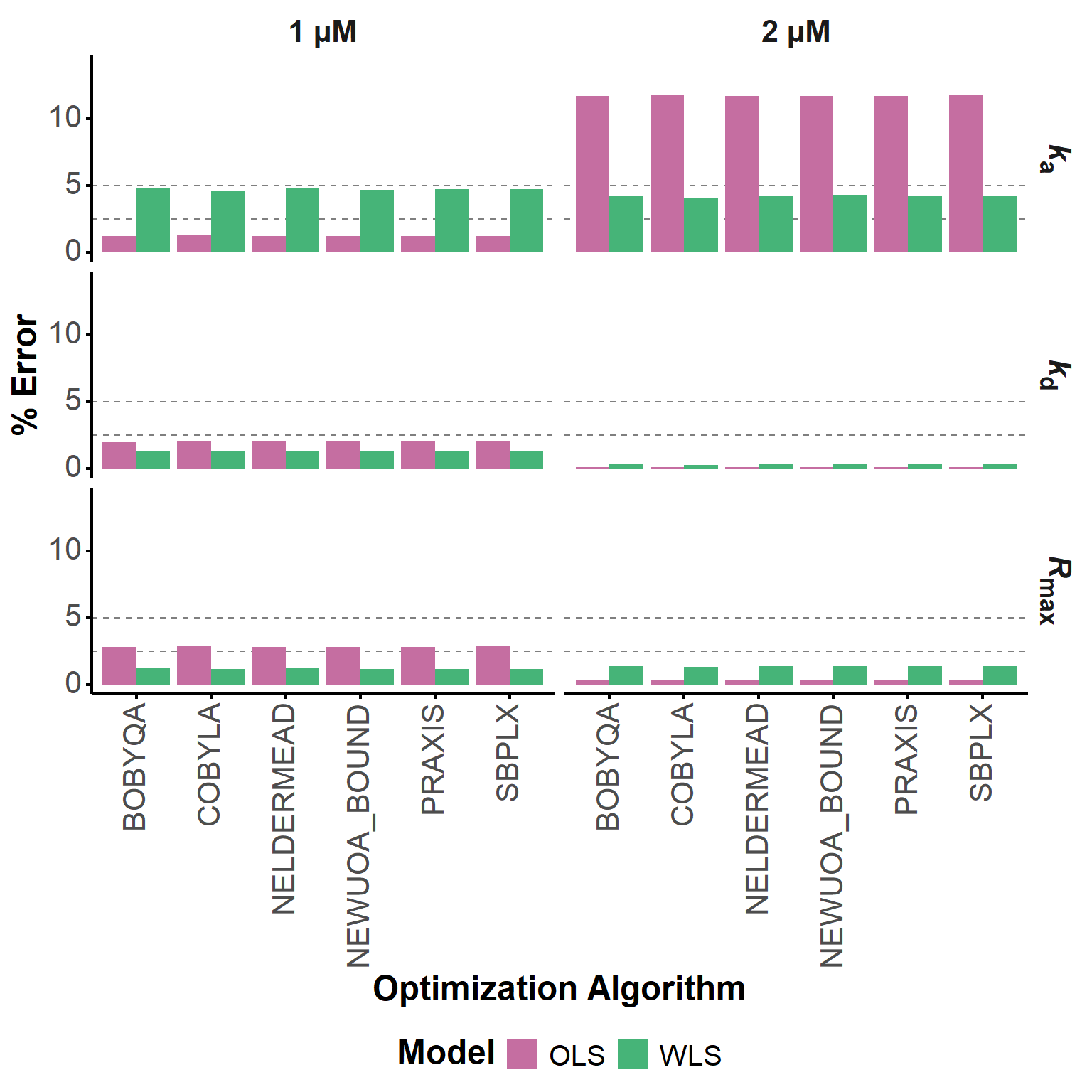
Overall, a combination of COBYLA with WLS gave the best results for the 1 and 2 µM experiments (Table 9), but, again, the differences are marginal and the workflow is robust to the choice of the optimization algorithm. In any case, the original choice of working with COBYLA is validated.
mean_errors <- algo_comp_param_store[experiment != "500 nM"] |>
  #change key to algorithm, model, param
  setkey(algorithm, model) |>
  _[, .(mean_error = mean(pct_error)), by = .(algorithm, model)] |>
  _[order(mean_error)] |>
  _[, algorithm := gsub("NLOPT_LN_", "", algorithm)]

mean_errors |>
  gt(groupname_col = "model") |>
  fmt_number(columns = "mean_error", decimals = 2) |>
  opt_row_striping() |>
  data_color(
    columns = "mean_error",
    colors = scales::col_numeric(
      palette = c("forestgreen", "white", "coral"),
      domain = c(min(mean_errors$mean_error)-0.01, max(mean_errors$mean_error)+0.01),
      na.color = "coral",
      alpha = 0.8
    )
  ) |>
  cols_label(
    algorithm = html("<b>Algorithm</b>"),
    mean_error = html("<b>Mean % Error</b>")
  ) |>
  # tab_header(title = html("<b>Algorithm Comparison: Parameter Estimation</b>")) |>
  tab_style(
    style = cell_text(weight = "bold"),
    locations = cells_row_groups()
)| Algorithm | Mean % Error |
|---|---|
| WLS | |
| COBYLA | 2.11 |
| SBPLX | 2.17 |
| PRAXIS | 2.17 |
| BOBYQA | 2.18 |
| NELDERMEAD | 2.18 |
| NEWUOA_BOUND | 2.19 |
| OLS | |
| BOBYQA | 3.02 |
| NEWUOA_BOUND | 3.02 |
| NELDERMEAD | 3.02 |
| PRAXIS | 3.03 |
| SBPLX | 3.05 |
| COBYLA | 3.06 |
source("R/realfit_waveRAPID.R")

final_realfit <- lapply(
  unique(long_dt$exp),
  function(experiment) {
    cat("Fitting experiment", experiment, "\n")
    fit_waveRAPID(
      sim_mck[[experiment]],
      real_data = long_dt[exp == experiment],
      Rmax_init_offset = 0.99,
      smooth_param = 0.5,
      lbd = 0,
      opt_algo = "NLOPT_LN_COBYLA",
      optimize_on_smooth = TRUE
    )
  }
)

names(final_realfit) <- unique(long_dt$exp)


p_final_realfit <- lapply(
  c("2 µM", "1 µM", "500 nM"),
  function(x){
    fit_plot(final_realfit[[x]], "fit") + ggtitle(paste(x))
  }) |>
  patchwork::wrap_plots() +
  plot_layout(ncol = 1, guides = "collect") &
  theme(legend.position = "bottom")
Figure 17 shows the final fits obtained with the optimized parameters for each experiment, using COBYLA as optimization algorithm. The fit quality is generally good, with a better fit of the dissociation phases when using WLS, as expected (Tables 10, 11, 12). The estimated kinetic parameters are in good agreement with the Biacore estimates, especially for the 1 and 2 µM experiments. For the 500 nM experiment, the estimation is less accurate, which could be due to a lower signal-to-noise ratio or other experimental factors affecting the data quality.
p_final_realfit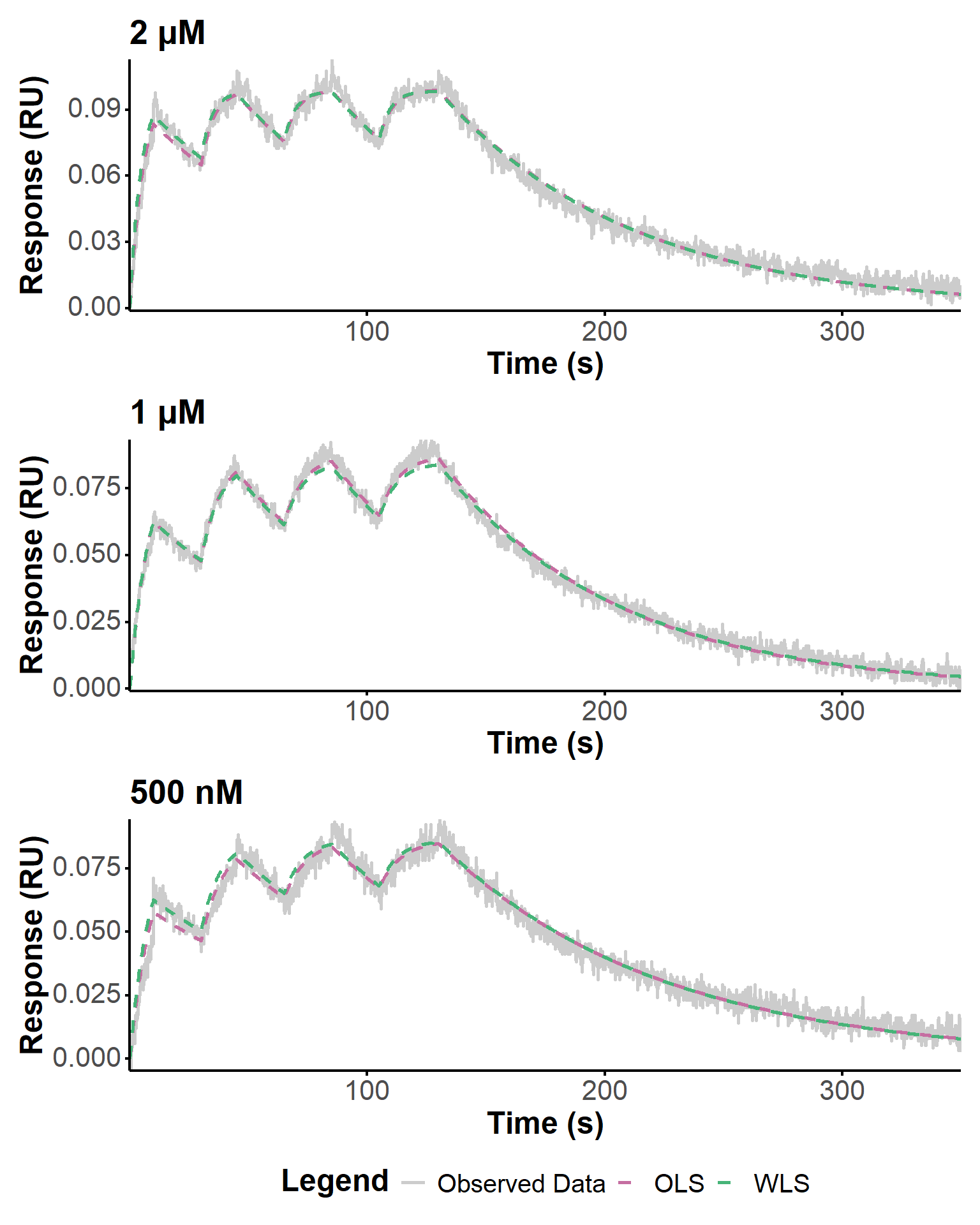
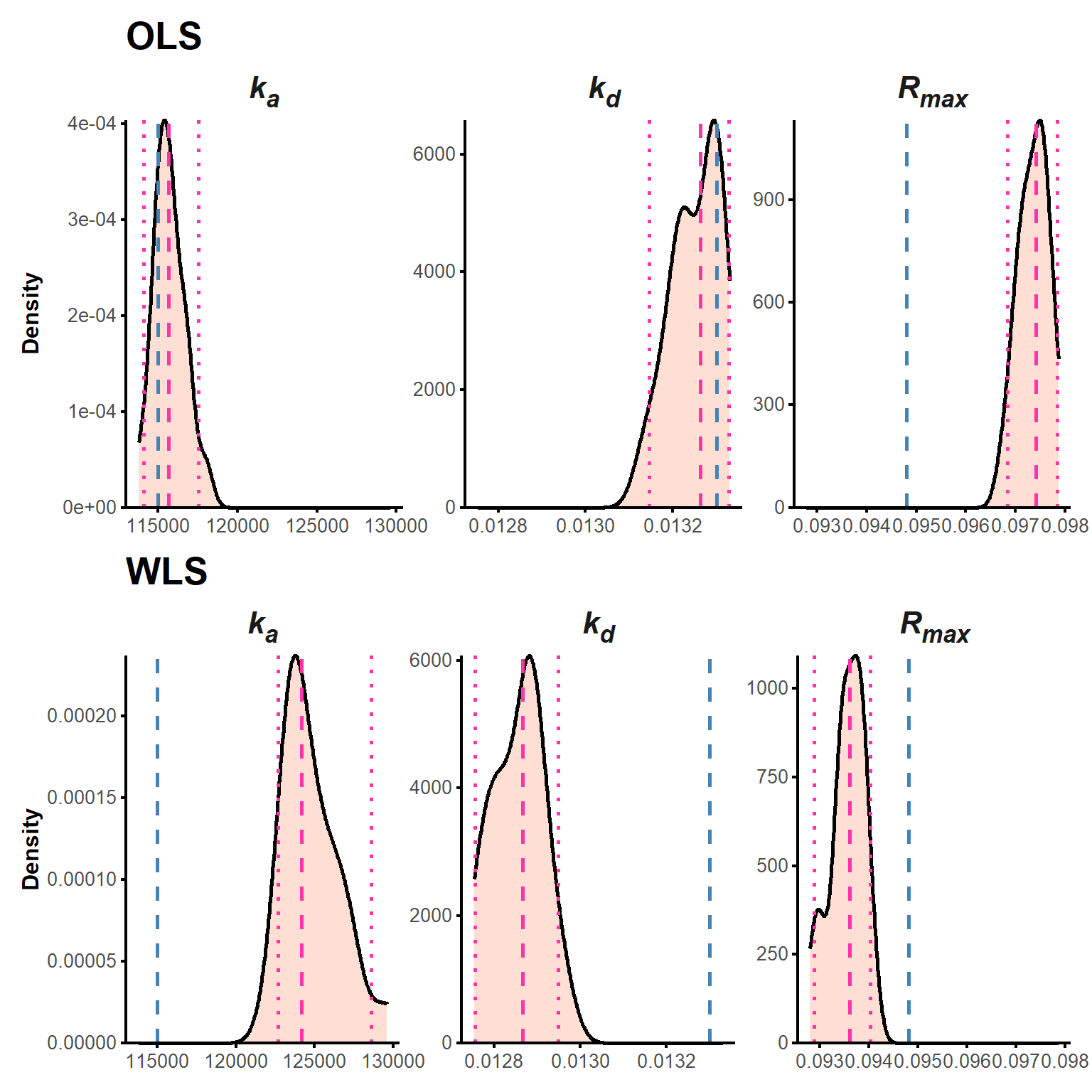
param_table(final_realfit[["2 µM"]])param_table(final_realfit[["1 µM"]])param_table(final_realfit[["500 nM"]])Here, we apply the bootstrapping procedure prepared with fake data (Section 2.3.2.2) to assess its effectiveness in evaluating the uncertainty in the estimated kinetic parameters with real data. We used 20 bootstrap replicates for each experiment to limit the computational burden. The results for the 1 µM experiment are shown below (Table 13, Figure 18). The distributions are rather narrow and confirm the robustness of our approach.
boot_real <- lapply(
  final_realfit,
  function(fit) {
    boot_waveRAPID(fit, n_boot = 20)
  }
)source("R/boot_waveRAPID.R")
param_table(boot_real[["1 µM"]])p_realboot1 <- plot(boot_real[["1 µM"]], "density") &
#rescale axis text smaller
theme(
axis.text = element_markdown(size = 10),
axis.title = element_markdown(size = 12),
legend.text = element_markdown(size = 10),
legend.title = element_markdown(size = 12)
)p_realboot1